


ISO/FDIS 5878
(Main)Reference atmospheres for aerospace use — Temperature profiles, wind characteristics and humidity models
General Information
- Abstract
Presents information on the seasonal, latidudinal, longitudinal and day-to-day variability of atmospheric properties at levels between the surface and 80 km. The systematic variation of atmospheric properties is shown for altitudes up to 80 km by a family of models, comprising the reference atmospheres tropical, sub-tropical, mid-latidude, sub-arctic and arctic. Furthermore temporal and spatial variations and frequency distributions of observed temperatures and densities are given.
- Status
- Not Published
- Technical Committee
- ISO/TC 20/SC 6 - Standard atmosphere
- Drafting Committee
- ISO/TC 20/SC 6 - Standard atmosphere
- Current Stage
- 5000 - FDIS registered for formal approval
- Start Date
- 06-May-2026
- Completion Date
- 13-May-2026
Buy Documents

ISO/FDIS 5878 - Reference atmospheres for aerospace use — Temperature profiles, wind characteristics and humidity models

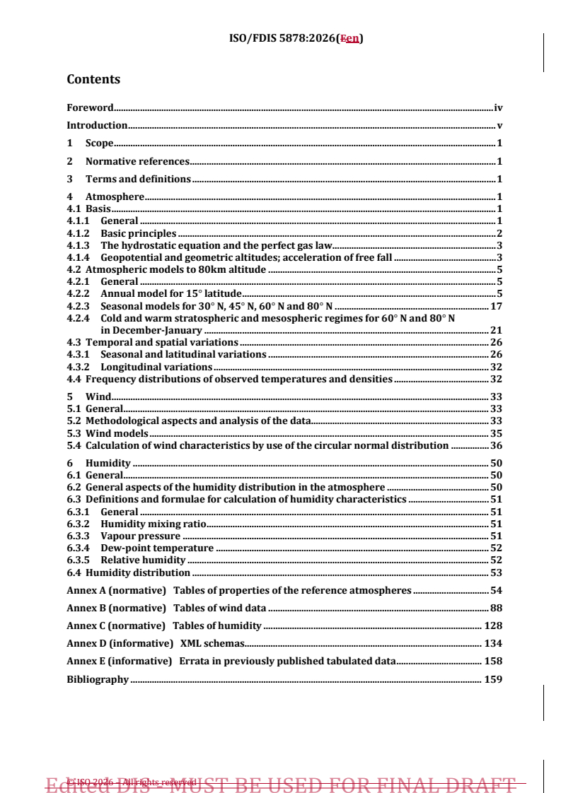

REDLINE ISO/FDIS 5878 - Reference atmospheres for aerospace use — Temperature profiles, wind characteristics and humidity models
Overview
ISO/FDIS 5878:2026 provides a comprehensive framework for reference atmospheres tailored to aerospace use, focusing on temperature profiles, wind characteristics, and humidity models. Developed by the International Organization for Standardization (ISO) through Technical Committee TC 20/SC 6, this international standard presents systematic data on meteorological parameters vital for aerospace engineering, flight operations, and atmospheric studies. The coverage extends from Earth’s surface up to 80 km, capturing latitudinal, longitudinal, seasonal, and day-to-day variations in atmospheric properties. This latest edition updates and unifies previous standards, ensuring alignment with recent developments in ISO 2533 and incorporating wind and humidity data for robust aerospace applications.
Key Topics
- Reference Atmospheres: The standard introduces a family of atmospheric models, each representing different climatic zones including tropical, sub-tropical, mid-latitude, sub-arctic, and arctic conditions. These models reflect typical atmospheric behavior across key latitudinal bands.
- Temperature and Density Profiles: Seasonal and regional variations in temperature and air density are presented through vertical profiles. These are critical for estimating aerodynamic heating, lift, and vehicle performance.
- Wind Characteristics: The document consolidates wind data relevant for aircraft routing, flight safety, and atmospheric transport analysis, presented in an accessible, averaged format across major world zones.
- Humidity Models: Recognizing the operational impact of atmospheric moisture, the standard details vertical humidity distributions, with emphasis on data up to 10 km where moisture has the greatest practical effects.
- Data Variability and Distribution: Statistical frequency distributions and temporal-spatial variability are documented, providing users with insight into the range of atmospheric conditions for risk assessment and robust design.
- Physical Assumptions: Calculations are rooted in fundamental equations such as the hydrostatic equation and the perfect gas law, making use of geopotential heights and accounting for gravity variations with latitude and altitude.
Applications
ISO/FDIS 5878 is vital for a range of aerospace and atmospheric applications, such as:
- Aerospace Vehicle Design: Engineers rely on accurate atmospheric models to simulate aircraft and spacecraft behavior, estimate aerodynamic loads, and define design criteria for structural integrity and performance.
- Operational Flight Planning: Pilots and air traffic planners use wind and temperature data to optimize flight paths, improve fuel efficiency, and schedule air routes in consideration of prevailing atmospheric conditions.
- Atmospheric Transport Studies: Environmental scientists and meteorologists employ these reference atmospheres to model pollutant dispersion, study climate impacts, and assess radiation transfer within different atmospheric layers.
- Aviation Safety: Understanding humidity and temperature profiles aids in evaluating icing risk, visibility, and the propagation of radio signals for communication and navigation.
- Standardized Benchmarking: Consistent reference data supports international harmonization for software simulation, regulatory compliance, and aerospace certification projects.
Related Standards
- ISO 2533:2026 Standard Atmosphere: The principal reference underpinning the calculations and definitions in ISO/FDIS 5878; establishes thermodynamic and physical constants for atmospheric modelling.
- Previous Editions of ISO 5878: The 2026 edition supersedes earlier versions, including ISO 5878:1982 and its addenda, consolidating and updating guidance on wind and humidity references.
- WMO and National Meteorological Standards: Complementary sources for observed atmospheric data and specialized regional models.
- Environmental and Meteorological Standards: For broader environmental modelling-such as ICAO Annexes regarding aviation meteorology, or ISO guidance on atmospheric sampling and air quality.
By adopting ISO/FDIS 5878, aerospace industries, meteorological agencies, and research organizations gain access to harmonized and validated atmospheric reference models. This ensures more accurate engineering, safer operations, and aligned scientific research-essential for progress in aerospace and atmospheric sciences.
Relations
- Effective Date
- 07-Jan-2025
- Effective Date
- 07-Jan-2025
- Revises
ISO 5878:1982/Add 1:1983 - Reference atmospheres for aerospace use — Addendum 1: Wind supplement - Effective Date
- 07-Jan-2025
- Effective Date
- 07-Jan-2025
Buy Documents
ISO/FDIS 5878 - Reference atmospheres for aerospace use — Temperature profiles, wind characteristics and humidity models
REDLINE ISO/FDIS 5878 - Reference atmospheres for aerospace use — Temperature profiles, wind characteristics and humidity models
Get Certified
Connect with accredited certification bodies for this standard

BSI Group
BSI (British Standards Institution) is the business standards company that helps organizations make excellence a habit.

Bureau Veritas
Bureau Veritas is a world leader in laboratory testing, inspection and certification services.

DNV
DNV is an independent assurance and risk management provider.
Sponsored listings
Frequently Asked Questions
ISO/FDIS 5878 is a draft published by the International Organization for Standardization (ISO). Its full title is "Reference atmospheres for aerospace use — Temperature profiles, wind characteristics and humidity models". This standard covers: Presents information on the seasonal, latidudinal, longitudinal and day-to-day variability of atmospheric properties at levels between the surface and 80 km. The systematic variation of atmospheric properties is shown for altitudes up to 80 km by a family of models, comprising the reference atmospheres tropical, sub-tropical, mid-latidude, sub-arctic and arctic. Furthermore temporal and spatial variations and frequency distributions of observed temperatures and densities are given.
Presents information on the seasonal, latidudinal, longitudinal and day-to-day variability of atmospheric properties at levels between the surface and 80 km. The systematic variation of atmospheric properties is shown for altitudes up to 80 km by a family of models, comprising the reference atmospheres tropical, sub-tropical, mid-latidude, sub-arctic and arctic. Furthermore temporal and spatial variations and frequency distributions of observed temperatures and densities are given.
ISO/FDIS 5878 is classified under the following ICS (International Classification for Standards) categories: 49.020 - Aircraft and space vehicles in general. The ICS classification helps identify the subject area and facilitates finding related standards.
ISO/FDIS 5878 has the following relationships with other standards: It is inter standard links to ISO 5878:1982/Add 2:1983, ISO 5878:1982, ISO 5878:1982/Add 1:1983, ISO 5878:1982/Amd 1:1990. Understanding these relationships helps ensure you are using the most current and applicable version of the standard.
ISO/FDIS 5878 is available in PDF format for immediate download after purchase. The document can be added to your cart and obtained through the secure checkout process. Digital delivery ensures instant access to the complete standard document.
Standards Content (Sample)
FINAL DRAFT
International
Standard
ISO/TC 20/SC 6
Reference atmospheres for
Secretariat: GOST R
aerospace use — Temperature
Voting begins on:
profiles, wind characteristics and
2026-09-21
humidity models
Voting terminates on:
2026-11-16
RECIPIENTS OF THIS DRAFT ARE INVITED TO SUBMIT,
WITH THEIR COMMENTS, NOTIFICATION OF ANY
RELEVANT PATENT RIGHTS OF WHICH THEY ARE AWARE
AND TO PROVIDE SUPPOR TING DOCUMENTATION.
IN ADDITION TO THEIR EVALUATION AS
BEING ACCEPTABLE FOR INDUSTRIAL, TECHNO
LOGICAL, COMMERCIAL AND USER PURPOSES, DRAFT
INTERNATIONAL STANDARDS MAY ON OCCASION HAVE
TO BE CONSIDERED IN THE LIGHT OF THEIR POTENTIAL
TO BECOME STAN DARDS TO WHICH REFERENCE MAY BE
MADE IN NATIONAL REGULATIONS.
Reference number
FINAL DRAFT
International
Standard
ISO/TC 20/SC 6
Reference atmospheres for
Secretariat: GOST R
aerospace use — Temperature
Voting begins on:
profiles, wind characteristics and
humidity models
Voting terminates on:
RECIPIENTS OF THIS DRAFT ARE INVITED TO SUBMIT,
WITH THEIR COMMENTS, NOTIFICATION OF ANY
RELEVANT PATENT RIGHTS OF WHICH THEY ARE AWARE
AND TO PROVIDE SUPPOR TING DOCUMENTATION.
© ISO 2026
IN ADDITION TO THEIR EVALUATION AS
All rights reserved. Unless otherwise specified, or required in the context of its implementation, no part of this publication may
BEING ACCEPTABLE FOR INDUSTRIAL, TECHNO
LOGICAL, COMMERCIAL AND USER PURPOSES, DRAFT
be reproduced or utilized otherwise in any form or by any means, electronic or mechanical, including photocopying, or posting on
INTERNATIONAL STANDARDS MAY ON OCCASION HAVE
the internet or an intranet, without prior written permission. Permission can be requested from either ISO at the address below
TO BE CONSIDERED IN THE LIGHT OF THEIR POTENTIAL
or ISO’s member body in the country of the requester.
TO BECOME STAN DARDS TO WHICH REFERENCE MAY BE
MADE IN NATIONAL REGULATIONS.
ISO copyright office
CP 401 • Ch. de Blandonnet 8
CH-1214 Vernier, Geneva
Phone: +41 22 749 01 11
Email: copyright@iso.org
Website: www.iso.org
Published in Switzerland Reference number
ii
Contents
Foreword . iv
Introduction . v
1 Scope . 1
2 Normative references . 1
3 Terms and definitions . 1
4 Atmosphere . 1
4.1 Basis . 1
4.1.1 General . 1
4.1.2 Basic principles . 2
4.1.3 The hydrostatic equation and the perfect gas law . 3
4.1.4 Geopotential and geometric altitudes; acceleration of free fall . 3
4.2 Atmospheric models to 𝟖𝟖𝟖𝟖𝟖𝟖𝟖𝟖 altitude . 5
4.2.1 General . 5
4.2.2 Annual model for 𝟏𝟏𝟏𝟏° latitude . 5
4.2.3 Seasonal models for 𝟑𝟑𝟖𝟖° N, 𝟒𝟒𝟏𝟏° N, 𝟔𝟔𝟖𝟖° N and 𝟖𝟖𝟖𝟖° N . 12
4.2.4 Cold and warm stratospheric and mesospheric regimes for 𝟔𝟔𝟖𝟖° N and 𝟖𝟖𝟖𝟖° N
in December-January . 15
4.3 Temporal and spatial variations . 18
4.3.1 Seasonal and latitudinal variations . 18
4.3.2 Longitudinal variations . 22
4.4 Frequency distributions of observed temperatures and densities . 22
5 Wind . 23
5.1 General . 23
5.2 Methodological aspects and analysis of the data. 23
5.3 Wind models . 25
5.4 Calculation of wind characteristics by use of the circular normal distribution . 26
6 Humidity . 34
6.1 General . 34
6.2 General aspects of the humidity distribution in the atmosphere . 34
6.3 Definitions and formulae for calculation of humidity characteristics . 35
6.3.1 General . 35
6.3.2 Humidity mixing ratio . 35
6.3.3 Vapour pressure . 35
6.3.4 Dew-point temperature . 36
6.3.5 Relative humidity . 36
6.4 Humidity distribution . 37
Annex A (normative) Tables of properties of the reference atmospheres . 38
Annex B (normative) Tables of wind data . 72
Annex C (normative) Tables of humidity . 111
Annex D (informative) XML schemas. 117
Annex E (informative) Errata in previously published tabulated data . 142
Bibliography . 143
iii
Foreword
ISO (the International Organization for Standardization) is a worldwide federation of national standards
bodies (ISO member bodies). The work of preparing International Standards is normally carried out
through ISO technical committees. Each member body interested in a subject for which a technical
committee has been established has the right to be represented on that committee. International
organizations, governmental and non-governmental, in liaison with ISO, also take part in the work. ISO
collaborates closely with the International Electrotechnical Commission (IEC) on all matters of
electrotechnical standardization.
The procedures used to develop this document and those intended for its further maintenance are
described in the ISO/IEC Directives, Part 1. In particular, the different approval criteria needed for the
different types of ISO document should be noted. This document was drafted in accordance with the
editorial rules of the ISO/IEC Directives, Part 2 (see www.iso.org/directives).
ISO draws attention to the possibility that the implementation of this document may involve the use of
(a) patent(s). ISO takes no position concerning the evidence, validity or applicability of any claimed
patent rights in respect thereof. As of the date of publication of this document, ISO had not received notice
of (a) patent(s) which may be required to implement this document. However, implementers are
cautioned that this may not represent the latest information, which may be obtained from the patent
database available at www.iso.org/patents. ISO shall not be held responsible for identifying any or all
such patent rights.
Any trade name used in this document is information given for the convenience of users and does not
constitute an endorsement.
For an explanation of the voluntary nature of standards, the meaning of ISO specific terms and
expressions related to conformity assessment, as well as information about ISO's adherence to the World
Trade Organization (WTO) principles in the Technical Barriers to Trade (TBT), see
www.iso.org/iso/foreword.html.
This document was prepared by Technical Committee ISO/TC 20, Aircraft and space vehicles, SC 6,
Standard atmosphere.
This second edition cancels and replaces the first edition (ISO 5878:1982), which has been technically
revised. It also incorporates the Addenda ISO 5878:1982/Add 1:1983, ISO 5878:1982/Add 2:1983 and
ISO 5878:1982/Amd 1:1990.
The major changes are as follows:
— calculations in this document have been updated to use the latest edition of ISO 2533:2026;
— all figures have been re-plotted in vector format to the accurate specifications of the models;
— all data tables have been moved to the annexes;
— an errata of tabulated data is included in Annex E.
Any feedback or questions on this document should be directed to the user’s national standards body. A
complete listing of these bodies can be found at www.iso.org/members.html.
iv © ISO 2026 – All rights reserved
Introduction
0.1 General
Understanding atmospheric characteristics is fundamental to numerous scientific and engineering
endeavours, particularly in aerospace, meteorology, and environmental sciences. The atmosphere’s
complex behaviour presents challenges for vehicle design, weather prediction, pollution transport
modelling, and aviation operations.
The need for standardized atmospheric models has grown with the advancement of aerospace
technology and increasing concerns about climate change. These models must balance accuracy with
usability, providing sufficient detail while remaining accessible to non-specialists.
This document presents three key aspects of atmospheric behaviour:
— Temperature and density profiles, which affect vehicle performance, aerodynamic heating, and
structural loads.
— Moisture content, which impacts visibility, icing conditions, and radio wave propagation.
— Wind patterns, which influence flight planning, fuel consumption, and transport of atmospheric
constituents.
These properties vary significantly with altitude, latitude, season, and geographic location, interacting to
form a complete picture of atmospheric behaviour necessary for modern applications.
The publication of this document as the second edition marks the 43rd anniversary of the reference
atmospheres for aerospace use, first published in 1982 and extended twice in 1983 to cover wind and
humidity data.
0.2 Temperature and density variations of the atmosphere
The characterization of atmospheric temperature and density variations represents one of the most
fundamental aspects of atmospheric modelling. The approach taken in this document employs a family
of reference models that capture the systematic variations across different latitudinal bands, from
tropical ( 15° ) to Arctic ( 80° N) regions. These models are constructed from extensive observational
data collected through various measurement techniques including radiosondes, meteorological rockets,
and other specialized atmospheric sensing systems.
The reference atmospheres account for both the regular patterns and special phenomena that occur in
different regions. In tropical areas, they capture the relatively stable annual conditions and characteristic
features like the trade wind inversion. In middle latitudes, they describe the significant seasonal
variations in temperature and density profiles. The models give particular attention to Arctic and sub-
Arctic regions, where sudden stratospheric warmings and other unique phenomena can produce
dramatic changes in atmospheric structure.
These models are founded on fundamental physical principles, including the hydrostatic equation and
perfect gas law, with careful consideration given to variations in gravity with latitude and altitude
through geopotential calculations. They provide not just mean conditions but also statistical distributions
of observed values, giving users insight into the variability they can encounter in real-world applications.
This comprehensive approach allows for realistic engineering design criteria while maintaining scientific
accuracy.
v
0.3 Wind characteristics
The wind patterns in Earth’s atmosphere emerge from complex interactions between thermal gradients,
pressure systems, surface conditions, and planetary rotation. These interactions create distinctive flow
patterns that vary systematically with latitude, altitude, and season, while also exhibiting significant local
and temporal variations. Understanding these patterns is crucial for applications ranging from aircraft
route planning to pollution dispersion modelling.
The meridional distribution of winds reveals a complex structure of atmospheric circulation. In tropical
latitudes, easterly components dominate the lower and middle troposphere, while subtropical regions
feature strong westerly flows and jet streams at 10km to 13km altitude. Temperate latitudes exhibit
wave-like westerly flows associated with mobile cyclone systems, and the stratosphere demonstrates
dramatic seasonal reversals in wind direction. This structure is further complicated by variations in wind
speed and direction with altitude, creating wind shear patterns that are particularly significant for
aviation and atmospheric transport.
While detailed wind data is available from various meteorological organizations, including the World
Meteorological Organization (WMO) and national weather services, the sheer volume and complexity of
this information can be overwhelming for practical applications. This document presents wind
characteristics in a simplified yet comprehensive format, averaging data over major regions while
retaining essential features of the atmospheric circulation patterns. This approach makes the information
more accessible to users who require wind data for specific applications but may not have extensive
meteorological expertise.
0.4 Moisture content
Atmospheric moisture, though a minor constituent by mass, plays a disproportionately large role in
atmospheric processes and human activities. The maximum water content of approximately 4% by mass
belies its crucial influence on weather patterns, climate systems, and aviation operations. Understanding
moisture distribution and variation is essential for applications ranging from aircraft design to weather
forecasting and climate modelling.
Water exists in all three phases within the atmosphere — vapor, liquid, and solid — each with distinct
implications for various applications. Water vapor, the primary focus of this document, affects air density,
radio wave propagation, and atmospheric stability. Liquid water in clouds and fog impacts visibility and
aircraft operations, while solid forms create icing hazards and affect precipitation patterns. The vertical
distribution of moisture is particularly significant, with the majority concentrated in the lower
atmosphere — 60% within the first 2km and 99% below 10km .
The quantification of atmospheric moisture through multiple measures — humidity mixing ratio, vapor
pressure, and dew-point temperature — provides users with flexible options for different applications.
These complementary measures allow for direct use in engineering calculations, meteorological analyses,
and practical operations. The data presented focuses on the lowest 10km of the atmosphere, where
reliable radiosonde measurements are available and where moisture content has the most significant
practical implications.
vi © ISO 2026 – All rights reserved
FINAL DRAFT International Standard ISO/FDIS 5878:2026(en)
Reference atmospheres for aerospace use — Temperature
profiles, wind characteristics and humidity models
1 Scope
This document presents comprehensive information on atmospheric properties and their variations from
Earth’s surface up to 80km , encompassing:
— seasonal, latitudinal, and longitudinal variability of temperature, pressure, and density;
— spatial distribution of wind characteristics;
— humidity values up to 10km above sea level, based on reliable radiosonde data.
The data and models are intended for use in aerospace design (such as aircraft performance evaluation),
operational planning (such as air route planning), and atmospheric transport studies (such as
atmospheric contaminant transport assessment).
2 Normative references
The following documents are referred to in the text in such a way that some or all of their content
constitutes requirements of this document. For dated references, only the edition cited applies. For
undated references, the latest edition of the referenced document (including any amendments) applies.
ISO 2533:2026, Standard atmosphere
3 Terms and definitions
For the purposes of this document, the terms and definitions given in ISO 2533:2026 apply.
ISO and IEC maintain terminology databases for use in standardization at the following addresses:
— ISO Online browsing platform: available at https://www.iso.org/obp
— IEC Electropedia: available at https://www.electropedia.org
4 Atmosphere
4.1 Basis
4.1.1 General
The systematic (latitudinal and seasonal) variation of atmospheric properties is shown for altitudes up
to 80km by a family of models, comprising the reference atmospheres in Table 1.
Table 1 — Reference atmospheres
Title Latitude Time of year
Tropical 15° Annual average
Sub-tropical 30° N June-July and December-January
Mid-latitude 45° N June-July and December-January
Sub-Arctic 60° N June-July and December-January
Cold and warm stratospheric-mesospheric regimes for December-January
Arctic 80° N Same as sub-Arctic
Some special considerations employed in the development of this family of reference atmospheres are
listed below:
a) With the exception of the 15° latitude model, the reference atmospheres are considered applicable
to the northern hemisphere only. However, it is believed that they closely approximate mid-latitude
conditions in the southern hemisphere.
b) The models are defined by temperature-altitude profiles in which the vertical gradients of
temperature are constant with respect to geopotential altitude within each of a number of layers.
c) The air is assumed to be a perfect gas, free from moisture and dust.
−1
d) The molar mass of dry air, 𝑀𝑀 = 28 964 420kgkmol , is assumed to be constant at altitudes up to
−1 −1
80km . The specific gas constant of dry air 𝑅𝑅 , is equal to 28 705 287JK kg (Table 2).
e) Characteristics such as the trade inversion in the tropics and the winter surface inversion in Arctic
and sub-Arctic regions are included in the models.
Table 2 — Main values used for the calculation of the reference atmospheres
Symbol Value Unit of measurement Description
−2
9,806 65 +0 ms standard acceleration of free fall
𝑔𝑔
n
−1
𝑀𝑀 2,896 442 +1 kgkmol molar mass of dry air at sea level
−1
6,022 140 760 Avogadro constant, as defined in the BIPM SI Brochure
𝑁𝑁
mol
A
-23
∗ −1 −1
8,314 32 +3 JK kmol or universal gas constant
𝑅𝑅
2 −2 −1 −1
kgm s K kmol
−1 −1 2 −1 −2
𝑅𝑅 2,870 528 7 specific gas constant
JK kg or m K s
+2
4.1.2 Basic principles
The numerical values for the various thermodynamic and physical quantities used in the computations
of atmospheric properties defined in ISO 2533:2026 shall apply, except for the following special
considerations:
a) surface conditions for each for the reference atmospheres are based on sea-level values of
temperature, pressure and density for the appropriate season and latitude
b) values of the acceleration of free fall at sea level for latitudes other than 45° were obtained from
Lambert’s equation (Formula (1), from Reference [41]) in which gravity varies with latitude 𝜑𝜑 .
2 −2
( )[ ]
𝑔𝑔 = 9,806 16 1− 0,002 637 3𝑐𝑐𝑐𝑐𝑐𝑐 2𝜑𝜑 + 0,000 005 9𝑐𝑐𝑐𝑐𝑐𝑐 2𝜑𝜑 ms (1)
0𝜑𝜑
2 © ISO 2026 – All rights reserved
where
𝑔𝑔 is the acceleration of free fall at sea level for latitude 𝜑𝜑 , expressed in metres per second squared
0𝜑𝜑
−2
( ms );
𝜑𝜑 is the latitude, expressed in degrees ( ° ).
Values from this relationship, along with surface temperatures and pressures, are given in Table A.1. For
45° N, values of 𝑔𝑔 and 𝑟𝑟 are taken from ISO 2533:2026.
0𝜑𝜑 𝜑𝜑
4.1.3 The hydrostatic equation and the perfect gas law
The hydrostatic equation and the perfect gas law defined in ISO 2533:2026, 4.2 shall apply.
4.1.4 Geopotential and geometric altitudes; acceleration of free fall
The geopotential and geometric altitudes, as well as the acceleration of free fall, defined in ISO 2533:2026,
4.3 shall apply.
Gravity is the vector sum of the gravitational attraction and the centrifugal force induced by the earth’s
rotation; it is therefore a complicated function of latitude and the radial distance from the centre of the
earth, and the expression for the acceleration of free fall is generally awkward and impractical. However,
allowance can be made for the centrifugal forces, with sufficient accuracy for these reference
atmospheres, by using a fictitious or nominal value of the earth’s radius, 𝑟𝑟 , at each latitude. The
𝜑𝜑
acceleration of free fall 𝑔𝑔 (ℎ) may be found for each height and latitude by use of 𝑟𝑟 , with Newton’s law
𝜑𝜑 𝜑𝜑
of gravitation as shown in Formula (2).
𝑟𝑟
𝜑𝜑
𝑔𝑔 (ℎ) =𝑔𝑔 � � (2)
𝜑𝜑 0𝜑𝜑
𝑟𝑟 +ℎ
𝜑𝜑
where
𝑟𝑟 is the nominal radius of the earth at a specific latitude, taken from Table A.1, expressed in metres ( m );
𝜑𝜑
𝑔𝑔 is the acceleration of free fall at sea level for latitude 𝜑𝜑 , expressed in metres per second squared
0𝜑𝜑
−2
( ms ).
( )
Integration of ISO 2533:2026, Formula 7, after substituting for 𝑔𝑔 ℎ from Formula (2), gives the
𝜑𝜑
relationship between geopotential and geometric altitudes in Formula (3) and Formula (4).
𝑟𝑟 ℎ 𝑔𝑔
𝜑𝜑 0𝜑𝜑
𝐻𝐻 = ⋅ (3)
𝑟𝑟 +ℎ 𝑔𝑔
𝜑𝜑 n
where
𝐻𝐻 is the geopotential altitude, expressed in metres ( m );
ℎ is the geometric altitude, expressed in metres ( m );
𝑔𝑔 is the acceleration of free fall at sea level for latitude 𝜑𝜑 , expressed in metres per second squared
0𝜑𝜑
−2
( ms );
𝑔𝑔 is the standard acceleration of free fall at mean sea level, expressed in metres per second squared
n
−2
( ms );
𝑟𝑟 is the nominal radius of the earth at a specific latitude, taken from Table A.1, expressed in metres ( m ).
𝜑𝜑
𝑟𝑟 𝐻𝐻
𝜑𝜑
ℎ = (4)
𝑔𝑔
0𝜑𝜑
𝑟𝑟 −𝐻𝐻
𝜑𝜑
𝑔𝑔
n
where
𝐻𝐻 is the geopotential altitude, expressed in metres ( m );
ℎ is the geometric altitude, expressed in metres ( m );
𝑔𝑔 is the acceleration of free fall at sea level for latitude 𝜑𝜑 , expressed in metres per second squared
0𝜑𝜑
−2
( ms );
𝑔𝑔 is the standard acceleration of free fall at mean sea level, expressed in metres per second squared
n
−2
( ms );
𝑟𝑟 is the nominal radius of the earth at a specific latitude, taken from Table A.1, expressed in metres ( m ).
𝜑𝜑
The radius 𝑟𝑟 is a fictitious quantity, the meaning of which may be explained in the following way: gravity,
𝜑𝜑
being the vector sum of the gravitational attraction and the centrifugal force induced by the earth’s
rotation, has a certain potential, the geopotential. This potential may be replaced by the potential of a
non-rotating homogeneous sphere in such a way that the gravitational attraction at the surface of the
sphere is equal to that at the earth’s surface both in magnitude and direction.
This condition is satisfied if the partial derivatives of 𝑔𝑔 , with respect to ℎ for ℎ = 0 in Formula (2) and
𝜑𝜑
in the more precise Formula (5) from reference Reference [41] are equal.
−6 −9
( ) ( )
𝑔𝑔 ℎ =𝑔𝑔 − 3,085 462 × 10 + 2,27 × 10 𝑐𝑐𝑐𝑐𝑐𝑐 2𝜑𝜑ℎ +
𝜑𝜑 0𝜑𝜑
−13 −15 2
( )
7,254 × 10 + 1,0 × 10 𝑐𝑐𝑐𝑐𝑐𝑐 2𝜑𝜑ℎ −
−19 −22 3
( )
1,517 × 10 + 6,0 × 10 𝑐𝑐𝑐𝑐𝑐𝑐 2𝜑𝜑ℎ (5)
where
ℎ is the geometric height, expressed in metres ( m );
−2
𝑔𝑔 is the acceleration of free fall, expressed in metres per second squared ( ms );
𝑔𝑔 is the acceleration of free fall at sea level for latitude 𝜑𝜑 , expressed in metres per second squared
0𝜑𝜑
−2
( ms );
𝜑𝜑 is the latitude, expressed in degrees ( ° );
𝑟𝑟 is the nominal radius of the earth at a specific latitude, taken from Table A.1, expressed in metres ( m ).
𝜑𝜑
The partial derivatives of 𝑔𝑔 , with respect to ℎ for ℎ = 0 are, from Formula (5), and described in Formula
𝜑𝜑
(6).
𝜕𝜕ℎ
𝜑𝜑
−6 −9
� � =−3,085 462 × 10 − 2,27 × 10 𝑐𝑐𝑐𝑐𝑐𝑐 2𝜑𝜑 (6)
𝜕𝜕ℎ
ℎ=0
where
ℎ is the geometric height, expressed in metres ( m );
−2
𝑔𝑔 is the acceleration of free fall, expressed in metres per second squared ( ms );
𝑔𝑔 is the acceleration of free fall at sea level for latitude 𝜑𝜑 , expressed in metres per second squared
0𝜑𝜑
−2
( ms );
𝜑𝜑 is the latitude, expressed in degrees ( ° );
𝑟𝑟 is the nominal radius of the earth at a specific latitude, taken from Table A.1, expressed in metres ( m ).
𝜑𝜑
And, together from Formula (2), we obtain Formula (7).
𝜕𝜕𝑔𝑔 2𝑔𝑔
𝜑𝜑 0𝜑𝜑
� � =− (7)
𝜕𝜕ℎ 𝑟𝑟
ℎ=0 𝜑𝜑
4 © ISO 2026 – All rights reserved
where
ℎ is the geometric height, expressed in metres ( m );
−2
𝑔𝑔 is the acceleration of free fall, expressed in metres per second squared ( ms );
𝑔𝑔 is the acceleration of free fall at sea level for latitude 𝜑𝜑 , expressed in metres per second squared
0𝜑𝜑
−2
( ms );
𝜑𝜑 is the latitude, expressed in degrees ( ° );
𝑟𝑟 is the nominal radius of the earth at a specific latitude, taken from Table A.1, expressed in metres ( m ).
𝜑𝜑
Equating the right-hand sides of Formula (6) and Formula (7), we have Formula (8).
𝑟𝑟 =𝑔𝑔 (8)
𝜑𝜑 0𝜑𝜑
−6 −9
3,085 462×10 +2,27×10 𝑐𝑐𝑐𝑐𝑐𝑐2𝜑𝜑
where
ℎ is the geometric height, expressed in metres ( m );
−2
𝑔𝑔 is the acceleration of free fall, expressed in metres per second squared ( ms );
𝑟𝑟 is the nominal radius of the earth at a specific latitude, taken from Table A.1, expressed in metres ( m );
𝜑𝜑
𝑔𝑔 is the acceleration of free fall at sea level for latitude 𝜑𝜑 , expressed in metres per second squared
0𝜑𝜑
−2
( ms ).
The values of 𝑟𝑟 , for the latitudes of the reference atmospheres are given in Table A.1.
𝜑𝜑
4.2 Atmospheric models to 𝟖𝟖𝟖𝟖𝟖𝟖𝟖𝟖 altitude
4.2.1 General
The reference atmospheres are defined by the vertical temperature profiles for each latitude and season
(see 4.1.1 b)).
Vertical pressure and density distributions were calculated from the temperature-altitude profiles using
the hydrostatic ISO 2533:2026, Formula 1 and the perfect gas law ISO 2533:2026, Formula 3 from 4.1
and the appropriate mean sea-level values of pressure.
Temperature and other properties of the reference atmospheres are given in Clause A.3. Brief
descriptions of seasonal, latitudinal, longitudinal and day-to-day variations of temperature and density
are included in 4.3.
A reference implementation of the computations defined in ISO 2533:2026 and this document is available
as the “atmospheris” open-source software library (Reference [42]). It provides algorithms for
calculating the atmosphere profile values (Clause A.3) and Rice distribution wind statistics (Table B.1)
from the empirical input parameters. The XML schema for the data tables is provided in Annex D.
4.2.2 Annual model for 𝟏𝟏𝟏𝟏° latitude
A mean annual atmosphere was adopted for 15° latitude as available observations indicate that the
seasonal variability of vertical profiles of temperature in the tropics is relatively small.
A mean annual temperature Profile (Figure 1) is based on observations taken at:
— Ascension ( 8° S, 14° W)
— Natal ( 6° S, 35° W)
— Ft. Sherman ( 9° N, 80° W)
— Kwajalein ( 9° N, 168° E)
— Antigua ( 17° N, 62° W)
— Guam ( 14° , 145° E)
— Grand Turk ( 21° N, 71° W)
— Research vessels Voyeikov and Shokalsky ( 20° S).
Features typical of the thermal structure of the tropical atmosphere are shown in Figure 1 and in Table
A.2.
EXAMPLE Routine averaging of monthly temperature-altitude data indicates an isothermal layer about
2km thick from 16km to 18km .
An examination of daily observations, however, reveals a sharp inversion at the tropopause. The sharp
inversion, a feature typical of the tropical atmosphere, has been retained and appears at 16,5km , the
mean annual altitude of the tropopause at 15° latitude.
The average altitude and magnitude of the trade wind inversion, a characteristic of the temperature
structure between 2km and 3km , over tropical ocean areas, have also been included in the 15° latitude
temperature-altitude profile.
6 © ISO 2026 – All rights reserved
a) Temperature-altitude profiles for the mean annual atmosphere for 𝟏𝟏𝟏𝟏° N latitude
b) Temperature-altitude profiles for the mean December-January and June-July atmospheres
for 𝟑𝟑𝟖𝟖° N latitude
8 © ISO 2026 – All rights reserved
c) Temperature-altitude profiles for the mean December-January and June-July atmospheres for
𝟒𝟒𝟏𝟏° N latitude
d) Temperature-altitude profiles for the mean December-January and June-July atmospheres
for 𝟔𝟔𝟖𝟖° N latitude
10 © ISO 2026 – All rights reserved
e) Temperature-altitude profiles for the mean December-January and June-July atmospheres
for 𝟖𝟖𝟖𝟖° N latitude
Key
X temperature (k)
Y geometric altitude (km)
1 annual mean
2 December-January
3 June-July
Figure 1 — Temperature-altitude profiles for the mean annual atmosphere for 𝟏𝟏𝟏𝟏° latitude and
for mean December-January and June-July atmospheres for 𝟑𝟑𝟖𝟖° N, 𝟒𝟒𝟏𝟏° N, 𝟔𝟔𝟖𝟖° N and 𝟖𝟖𝟖𝟖° N
4.2.3 Seasonal models for 𝟑𝟑𝟖𝟖° N, 𝟒𝟒𝟏𝟏° N, 𝟔𝟔𝟖𝟖° N and 𝟖𝟖𝟖𝟖° N
Temperature-altitude profiles for the mean December-January and June-July atmospheres for 30° N,
45° N, 60° N and 80° N are presented in Figure 1 and Clause A.4.
They are based on the temperature-altitude cross-sections in Figure 2. The temperature distributions
shown in Figure 2 for levels below 30km were derived from routine radiosonde observations.
12 © ISO 2026 – All rights reserved
Key
X latitude
Y geometric altitude (km)
A December-January
B June-July
1 Research vessel
2 Natal
3 Ascension
4 Ft. Sherman
5 Guam
6 Antigua Grand Turk
7 Barking Sands
8 Cp. Kennedy
9 Eglin
10 Woomera White Sands
11 Pt. Mugu
12 Wallops Island
13 Volgograd
14 Primrose Lake
15 West Geirinish
16 Ft. Churchill
17 Ft. Greely
18 Pt. Barrow
19 Thule
20 Heiss Island
Figure 2 — Temperature-altitude cross-sections for December-January and June-July
Mean northern hemisphere values were computed at various latitudes from available summaries
Reference [38] by giving equal weight to observed and interpolated temperature data at each 10° of
longitude (spatial averaging across longitudes). The initial pressures (sea-level values for each
atmosphere) were obtained from monthly normal sea-level charts (Reference [23],
USWB Tech. Paper No. 21) of the northern hemisphere.
The temperature field between 30km and 50km is based on meteorological rocket measurements taken
at locations shown in Table A.19. Instrumentation consists primarily of parachute-borne telemetering
sets with temperature-sensing elements (bead thermistors or resistance wires). Thermistor
measurements are subject to large corrections and uncertainties above 50km . Consequently the
thermistor data are used only for altitudes up to 50km . The temperature distributions between
50km and 80km are based primarily on grenade, falling sphere and pressure gauge experiments taken at
locations shown in Table A.20.
For temporal averaging of temperature observations, median rather than mean values are used since
bimodal distributions of temperature occur at high latitudes in winter in the upper stratosphere and
mesosphere. At other times and locations, distributions are nearly normal and the choice of median
versus mean has minimal impact. Dates of observation for the southern hemisphere were adjusted by six
months to conform to northern hemisphere seasons.
14 © ISO 2026 – All rights reserved
4.2.4 Cold and warm stratospheric and mesospheric regimes for 𝟔𝟔𝟖𝟖° N and 𝟖𝟖𝟖𝟖° N in December-
January
In Arctic and sub-Arctic regions, sudden warmings and coolings of the winter stratosphere and
mesosphere produce large changes in the vertical structure of the atmosphere. The magnitude and
altitude of maximum temperature change during major warmings and coolings vary considerably. Some
of the largest changes have been observed in the upper stratosphere. The winter temperature
distributions in this region are bimodal and temperatures are normally much lower or much higher than
the seasonal mean. Observed 35km temperatures, for example, have a range of roughly 75K in winter
compared with 20K in summer. Consequently, mean monthly or seasonal atmospheric models for the
winter months are of limited value for specifying the temperature in Arctic and sub-Arctic regions as the
day-to-day variations in temperature at many levels in the stratosphere are as great as or greater than
seasonal or latitudinal changes.
Vertical temperature profiles representative of the cold and warm stratospheric regimes that occur at
60° N and 80° N in December and January are shown in Figure 3 and Clause A.6.
a) Temperature-altitude profile for warm and cold for December-January atmospheres at 𝟔𝟔𝟖𝟖° N
16 © ISO 2026 – All rights reserved
Key
X temperature (k)
Y geometric altitude (km)
A 60° N Winter
B 80° N Winter
1 cold
2 mean
3 warm
b) Temperature-altitude profile for warm and cold for December-January atmospheres at 𝟖𝟖𝟖𝟖° N
Figure 3 — Temperature-altitude profiles for warm and cold for December-January
atmospheres at 𝟔𝟔𝟖𝟖° N and 𝟖𝟖𝟖𝟖° N
The profiles for the warm and cold models at 60° N and 80° N were constructed from temperatures
derived from radiosonde, rocket-sonde and grenade observations taken at:
— Ft. Greely, Alaska ( 64° N, 146° W)
— Ft. Churchill, Canada ( 59° N, 94° W)
— West Geirinish, Scotland ( 57° N, 7° W)
The 80° N models are based on observations taken at:
— Heiss Island ( 81° N, 58° E).
The warm regimes are arbitrarily defined as periods when the observed temperature at 45km is within
±2K of 267K , a value which is equalled or exceeded in 1% , 5% , 20% and 30% of the observations at Ft.
Greely, Ft. Churchill, West Geirinish and Heiss Island, respectively.
The cold regimes are defined as periods when the observed temperature at 45km at 60° N is within
±2K of 223K , and that at 80° N is within ±2K of 232K . The temperature of 223K is equalled or exceeded
in 98% , 95% , and 93% of the observations at West Geirinish, Ft. Churchill and Ft. Greely respectively,
and 232K is exceeded in 80% of the observations from Heiss Island ( 223K is equalled or exceeded
90% of the time at Heiss Island).
NOTE The definitions of warm and cold regimes in this model differ from their counterparts defined in the
Sudden Stratospheric Warming (SSW) literature [56].
Individual temperature soundings taken at Ft. Churchill, Ft. Greely, West Geirinish and Heiss Island which
satisfied the temperature requirements for a particular model at 45km were averaged together to obtain
a mean temperature-altitude profile between 8km and 80km . Mean seasonal conditions were assumed
below 9km as the vertical temperature profiles that emerged at these levels were not significantly
different from those for the mean seasonal conditions at 60° N and 80° N.
Locations and dates of soundings used in the construction of the warm and cold models are given in
Clause A.7. Due to the sparsity of data above 30km in Arctic and sub-Arctic regions, the frequencies of
occurrence of the warm and cold models at the various locations are rough estimates.
4.3 Temporal and spatial variations
4.3.1 Seasonal and latitudinal variations
Maximum and minimum mean monthly temperatures between the surface and 80km do not occur at all
latitudes and levels in the same month or season. Consequently, the tabulated temperatures for the
December-January and June-July reference atmospheres for 30° N, 45° N, 60° N and 80° N (Table A.25)
do not represent extreme seasonal temperatures at all altitudes. Nevertheless, they do provide a good
indication of the magnitude of the seasonal and latitudinal temperature variability that can be expected
at levels between the surface and 80km .
The maximum and minimum mean seasonal densities and pressures between the surface and 80km ,
however, normally occur in the June-July and December-January periods respectively between latitudes
30° N and 80° N (Table A.26).
At locations between 30° N and 80° N, maximum mean monthly temperatures at levels below
25km usually occur in June or July, and the minima in December or January. In the upper stratosphere,
18 © ISO 2026 – All rights reserved
however, semi-annual and biennial cycles complicate the annual temperature cycle. The magnitude of the
annual cycle is largest near the poles, decreasing toward the equator. The semi-annual and biennial cycles
are greatest near the equator, decreasing toward the poles. The phases as well as the amplitudes of these
temperature oscillations change with latitude and altitude. At middle and high latitudes, the annual and
semi-annual cycles tend to obscure the biennial oscillations.
Observations show that the semi-annual oscillation produces two pronounced maxima and minima
within the annual stratospheric temperature cycle in tropical and sub-tropical regions. North of
25° latitude, the combined annual and semi-annual components occasionally shift the time of maximum
temperature in the upper stratosphere to early June or May, and the minimum temperature to early
December or November.
However, in cases where the maximum mean monthly stratospheric temperatures occur in May rather
than June or July and the minimum in November rather than December or January, the differences
between May and June and November and December values are only a few degrees. In the mesosphere,
above 60km — 65km , the maximum mean monthly temperatures generally occur in December or
January, and the minimum in June or July. An exception occurs at Heiss Island, where maximum
temperatures are observed in late November and early December.
The vertical distribution of density is shown for the 15° latitude mean annual atmosphere and the
December-January and June-July atmospheres for 30° N, 45° N, 60° N and 80° N in Figure 4 as percentage
departures from the ISA densities defined in ISO 2533:2026. The maximum mean monthly densities at
levels between 10km and 80km and latitudes 30° N to 80° N occur in June or July, and minimum values
in December or January. Near the surface, pressures are usually highest in winter and lowest in summer.
The level of minimum seasonal variability of density near 8km represents the first isopycnic level where
density remains relatively constant throughout the year regardless of geographic location. The levels of
maximum seasonal and latitudinal variability in density and pressure are between 65km and 75km , and
the variability is greatest at high latitudes.
a) Departures of reference atmosphere densities for 𝟏𝟏𝟏𝟏° N (annual), 𝟑𝟑𝟖𝟖° (Dec-Jan, Jun-Jul) and
𝟒𝟒𝟏𝟏° N (Dec-Jan, Jun-Jul)
20 © ISO 2026 – All rights reserved
b) Departures of reference atmosphere densities for 𝟔𝟔𝟖𝟖° N (Dec-Jan, Jun-Jul), 𝟖𝟖𝟖𝟖° N (Dec-Jan,
Jun-Jul)
Key
X departure from standard (%)
Y geometric altitude (km)
1 annual
2 December-January
3 June-July
4 warm
5 mean
6 cold
Figure 4 — Departures of reference atmosphere densities (mean values from Clause A.3)
4.3.2 Longitudinal variations
In summer, longitudinal variations in the structure of the atmosphere are relatively small at all latitudes
compared with seasonal and latitudinal changes for levels up to 80km . Isotherms and contour lines of
constant-pressure charts in the stratosphere and mesosphere parallel the latitude circles, and the
associated circulation pattern is symmetrical about the poles. During the winter season, changes with
longitude remain small at low latitudes but become as important as those with latitude and season in
Arctic and sub-Arctic regions (from ESSA Tech. Rpt. WB 2, ESSA Tech. Rpt. WB
...
Date: 2026-04-15 07-29
Reference number of project: ISO/FDIS 5878 :2026(en)
Committee identification: TC 20/SC 6
Secretariat: GOST
Reference atmospheres for aerospace use — Temperature
profiles, wind characteristics and humidity models
Atmosphères de référence pour l’application aérospatiale — Profils de température,
caractéristiques du vent et modèles d’humidité
All rights reserved. Unless otherwise specified, or required in the context of its implementation, no
part of this publication may be reproduced or utilized otherwise in any form or by any means,
electronic or mechanical, including photocopying, or posting on the internet or an intranet, without
prior written permission. Permission can be requested from either ISO at the address below or
ISO’s member body in the country of the requester.
ISO copyright office
CP 401 • Ch. de Blandonnet 8
CH-1214 Vernier, Geneva
Phone: +41 22 749 01 11
Email: copyright@iso.org
Website: www.iso.org
Published in Switzerland
Contents
Foreword . iv
Introduction . v
1 Scope . 1
2 Normative references . 1
3 Terms and definitions . 1
4 Atmosphere . 1
4.1 Basis . 1
4.1.1 General . 1
4.1.2 Basic principles . 2
4.1.3 The hydrostatic equation and the perfect gas law . 3
4.1.4 Geopotential and geometric altitudes; acceleration of free fall . 3
4.2 Atmospheric models to 𝟖𝟖𝟖𝟖𝟖𝟖𝟖𝟖 altitude . 5
4.2.1 General . 5
4.2.2 Annual model for 𝟏𝟏𝟏𝟏° latitude . 5
4.2.3 Seasonal models for 𝟑𝟑𝟖𝟖° N, 𝟒𝟒𝟏𝟏° N, 𝟔𝟔𝟖𝟖° N and 𝟖𝟖𝟖𝟖° N . 17
4.2.4 Cold and warm stratospheric and mesospheric regimes for 𝟔𝟔𝟖𝟖° N and 𝟖𝟖𝟖𝟖° N
in December-January . 21
4.3 Temporal and spatial variations . 26
4.3.1 Seasonal and latitudinal variations . 26
4.3.2 Longitudinal variations . 32
4.4 Frequency distributions of observed temperatures and densities . 32
5 Wind . 33
5.1 General . 33
5.2 Methodological aspects and analysis of the data. 33
5.3 Wind models . 35
5.4 Calculation of wind characteristics by use of the circular normal distribution . 36
6 Humidity . 50
6.1 General . 50
6.2 General aspects of the humidity distribution in the atmosphere . 50
6.3 Definitions and formulae for calculation of humidity characteristics . 51
6.3.1 General . 51
6.3.2 Humidity mixing ratio . 51
6.3.3 Vapour pressure . 51
6.3.4 Dew-point temperature . 52
6.3.5 Relative humidity . 52
6.4 Humidity distribution . 53
Annex A (normative) Tables of properties of the reference atmospheres . 54
Annex B (normative) Tables of wind data . 88
Annex C (normative) Tables of humidity . 128
Annex D (informative) XML schemas. 134
Annex E (informative) Errata in previously published tabulated data . 158
Bibliography . 159
Foreword
ISO (the International Organization for Standardization) is a worldwide federation of national standards
bodies (ISO member bodies). The work of preparing International Standards is normally carried out
through ISO technical committees. Each member body interested in a subject for which a technical
committee has been established has the right to be represented on that committee. International
organizations, governmental and non-governmental, in liaison with ISO, also take part in the work. ISO
collaborates closely with the International Electrotechnical Commission (IEC) on all matters of
electrotechnical standardization.
The procedures used to develop this document and those intended for its further maintenance are
described in the ISO/IEC Directives, Part 1. In particular, the different approval criteria needed for the
different types of ISO document should be noted. This document was drafted in accordance with the
editorial rules of the ISO/IEC Directives, Part 2 (see www.iso.org/directives).
ISO draws attention to the possibility that the implementation of this document may involve the use of
(a) patent(s). ISO takes no position concerning the evidence, validity or applicability of any claimed
patent rights in respect thereof. As of the date of publication of this document, ISO had not received notice
of (a) patent(s) which may be required to implement this document. However, implementers are
cautioned that this may not represent the latest information, which may be obtained from the patent
database available at www.iso.org/patents. ISO shall not be held responsible for identifying any or all
such patent rights.
Any trade name used in this document is information given for the convenience of users and does not
constitute an endorsement.
For an explanation of the voluntary nature of standards, the meaning of ISO specific terms and
expressions related to conformity assessment, as well as information about ISO’sISO's adherence to the
World Trade Organization (WTO) principles in the Technical Barriers to Trade (TBT), see
www.iso.org/iso/foreword.html.
This document was prepared by Technical Committee ISO/TC 20, Aircraft and space vehicles, SC 6,
Standard atmosphere.
This second edition cancels and replaces the first edition (ISO 5878:1982), which has been technically
revised. It also incorporates the Addenda ISO 5878:1982/Add 1:1983, ISO 5878:1982/Add 2:1983 and
.ISO 5878:1982/Amd 1:1990.
The major changes are as follows:
— all content from has been incorporated, namely the wind model and its data tables;
— all content from has been incorporated, namely the humidity model and its data tables;
— calculations in this document have been updated to use the latest edition of ISO 2533:2026;
— all figures have been re-plotted in vector format to the accurate specifications of the models;
— all data tables have been moved to the annexes.;
An— an errata of previously published tabulated data is included in Annex E.
Any feedback or questions on this document should be directed to the user’s national standards body. A
complete listing of these bodies can be found at www.iso.org/members.html.
Introduction
0.1 General
Understanding atmospheric characteristics is fundamental to numerous scientific and engineering
endeavours, particularly in aerospace, meteorology, and environmental sciences. The atmosphere’s
complex behaviour presents challenges for vehicle design, weather prediction, pollution transport
modelling, and aviation operations.
The need for standardized atmospheric models has grown with the advancement of aerospace
technology and increasing concerns about climate change. These models must balance accuracy with
usability, providing sufficient detail while remaining accessible to non-specialists.
This document presents three key aspects of atmospheric behaviour:
— Temperature and density profiles, which affect vehicle performance, aerodynamic heating, and
structural loads.
— Moisture content, which impacts visibility, icing conditions, and radio wave propagation.
— Wind patterns, which influence flight planning, fuel consumption, and transport of atmospheric
constituents.
These properties vary significantly with altitude, latitude, season, and geographic location, interacting to
form a complete picture of atmospheric behaviour necessary for modern applications.
The publication of this document as the second edition marks the 43rd anniversary of the reference
atmospheres for aerospace use, first published in 1982 and extended twice in 1983 to cover wind and
humidity data.
0.2 Temperature and density variations of the atmosphere
The characterization of atmospheric temperature and density variations represents one of the most
fundamental aspects of atmospheric modelling. The approach taken in this document employs a family
of reference models that capture the systematic variations across different latitudinal bands, from
tropical ( 15° ) to Arctic ( 80° N) regions. These models are constructed from extensive observational
data collected through various measurement techniques including radiosondes, meteorological rockets,
and other specialized atmospheric sensing systems.
The reference atmospheres account for both the regular patterns and special phenomena that occur in
different regions. In tropical areas, they capture the relatively stable annual conditions and characteristic
features like the trade wind inversion. In middle latitudes, they describe the significant seasonal
variations in temperature and density profiles. The models give particular attention to Arctic and sub-
Arctic regions, where sudden stratospheric warmings and other unique phenomena can produce
dramatic changes in atmospheric structure.
These models are founded on fundamental physical principles, including the hydrostatic equation and
perfect gas law, with careful consideration given to variations in gravity with latitude and altitude
through geopotential calculations. They provide not just mean conditions but also statistical distributions
of observed values, giving users insight into the variability they can encounter in real-world applications.
This comprehensive approach allows for realistic engineering design criteria while maintaining scientific
accuracy.
0.3 Wind characteristics
The wind patterns in Earth’s atmosphere emerge from complex interactions between thermal gradients,
pressure systems, surface conditions, and planetary rotation. These interactions create distinctive flow
patterns that vary systematically with latitude, altitude, and season, while also exhibiting significant local
and temporal variations. Understanding these patterns is crucial for applications ranging from aircraft
route planning to pollution dispersion modelling.
The meridional distribution of winds reveals a complex structure of atmospheric circulation. In tropical
latitudes, easterly components dominate the lower and middle troposphere, while subtropical regions
feature strong westerly flows and jet streams at 10km to 13km altitude. Temperate latitudes exhibit
wave-like westerly flows associated with mobile cyclone systems, and the stratosphere demonstrates
dramatic seasonal reversals in wind direction. This structure is further complicated by variations in wind
speed and direction with altitude, creating wind shear patterns that are particularly significant for
aviation and atmospheric transport.
While detailed wind data is available from various meteorological organizations, including the World
Meteorological Organization (WMO) and national weather services, the sheer volume and complexity of
this information can be overwhelming for practical applications. This document presents wind
characteristics in a simplified yet comprehensive format, averaging data over major regions while
retaining essential features of the atmospheric circulation patterns. This approach makes the information
more accessible to users who require wind data for specific applications but may not have extensive
meteorological expertise.
0.4 Moisture content
Atmospheric moisture, though a minor constituent by mass, plays a disproportionately large role in
atmospheric processes and human activities. The maximum water content of approximately 4% by mass
belies its crucial influence on weather patterns, climate systems, and aviation operations. Understanding
moisture distribution and variation is essential for applications ranging from aircraft design to weather
forecasting and climate modelling.
Water exists in all three phases within the atmosphere — vapor, liquid, and solid — each with distinct
implications for various applications. Water vapor, the primary focus of this document, affects air density,
radio wave propagation, and atmospheric stability. Liquid water in clouds and fog impacts visibility and
aircraft operations, while solid forms create icing hazards and affect precipitation patterns. The vertical
distribution of moisture is particularly significant, with the majority concentrated in the lower
atmosphere — 60% within the first 2km and 99% below 10km .
The quantification of atmospheric moisture through multiple measures — humidity mixing ratio, vapor
pressure, and dew-point temperature — provides users with flexible options for different applications.
These complementary measures allow for direct use in engineering calculations, meteorological analyses,
and practical operations. The data presented focuses on the lowest 10km of the atmosphere, where
reliable radiosonde measurements are available and where moisture content has the most significant
practical implications.
FINAL DRAFT International Standard ISO/FDIS 5878:2026(en)
Reference atmospheres for aerospace use — Temperature
profiles, wind characteristics and humidity models
1 Scope
This document presents comprehensive information on atmospheric properties and their variations from
Earth’s surface up to 80km , encompassing:
— seasonal, latitudinal, and longitudinal variability of temperature, pressure, and density;
— spatial distribution of wind characteristics;
— humidity values up to 10km above sea level, based on reliable radiosonde data.
The data and models are intended for use in aerospace design (such as aircraft performance evaluation),
operational planning (such as air route planning), and atmospheric transport studies (such as
atmospheric contaminant transport assessment).
2 Normative references
The following documents are referred to in the text in such a way that some or all of their content
constitutes requirements of this document. For dated references, only the edition cited applies. For
undated references, the latest edition of the referenced document (including any amendments) applies.
ISO 2533:2026, Standard atmosphere
3 Terms and definitions
For the purposes of this document, the terms and definitions given in ISO 2533:2026 apply.
ISO and IEC maintain terminology databases for use in standardization at the following addresses:
— ISO Online browsing platform: available at https://www.iso.org/obp
— IEC Electropedia: available at https://www.electropedia.org
4 Atmosphere
4.1 Basis
4.1.1 General
The systematic (latitudinal and seasonal) variation of atmospheric properties is shown for altitudes up
to 80km by a family of models, comprising the reference atmospheres in Table 1.
Table 1 — Reference atmospheres
Title Latitude Time of year
Tropical 15° Annual average
Sub-tropical 30° N June-July and December-January
Mid-latitude 45° N June-July and December-January
Sub-Arctic 60° N June-July and December-January
Cold and warm stratospheric-mesospheric regimes for December-January
Arctic 80° N Same as sub-Arctic
Some special considerations employed in the development of this family of reference atmospheres are
listed below:
a) With the exception of the 15° latitude model, the reference atmospheres are considered applicable
to the northern hemisphere only. However, it is believed that they closely approximate mid-latitude
conditions in the southern hemisphere.
b) The models are defined by temperature-altitude profiles in which the vertical gradients of
temperature are constant with respect to geopotential altitude within each of a number of layers.
c) The air is assumed to be a perfect gas, free from moisture and dust.
−1
d) The molar mass of dry air, 𝑀𝑀 = 28 964 420kgkmol , is assumed to be constant at altitudes up to
−1 −1
kg (Table 2).
80km . The specific gas constant of dry air 𝑅𝑅 , is equal to 28 705 287JK
e) Characteristics such as the trade inversion in the tropics and the winter surface inversion in Arctic
and sub-Arctic regions are included in the models.
Table 2 — Main values used for the calculation of the reference atmospheres
Symbol Value Unit of measurement Description
−2
9,806 65 +0 ms standard acceleration of free fall
𝑔𝑔
n
−1
𝑀𝑀 2,896 442 +1 kgkmol molar mass of dry air at sea level
−1
6,022 140 760 Avogadro constant, as defined in the BIPM SI Brochure
𝑁𝑁
mol
A
-23
∗ −1 −1
8,314 32 +3 JK kmol or universal gas constant
𝑅𝑅
2 −2 −1 −1
kgm s K kmol
−1 −1 2 −1 −2
𝑅𝑅 2,870 528 7 specific gas constant
JK kg or m K s
+2
4.1.2 Basic principles
The numerical values for the various thermodynamic and physical quantities used in the computations
of atmospheric properties defined in ISO 2533:2026 shall apply, except for the following special
considerations:
a) surface conditions for each for the reference atmospheres are based on sea-level values of
temperature, pressure and density for the appropriate season and latitude
b) values of the acceleration of free fall at sea level for latitudes other than 45° were obtained from
Lambert’s equation (Formula (1), from Reference [41]) in which gravity varies with latitude 𝜑𝜑 .
2 −2
( )[ ]
𝑔𝑔 = 9,806 16 1− 0,002 637 3𝑐𝑐𝑐𝑐𝑐𝑐 2𝜑𝜑 + 0,000 005 9𝑐𝑐𝑐𝑐𝑐𝑐 2𝜑𝜑 ms (1)
0𝜑𝜑
where
𝑔𝑔 is the acceleration of free fall at sea level for latitude 𝜑𝜑 , expressed in metres per second squared
0𝜑𝜑
−2
( ms );
𝜑𝜑 is the latitude, expressed in degrees ( ° ).
Values from this relationship, along with surface temperatures and pressures, are given in Table A.1. For
45° N, values of 𝑔𝑔 and 𝑟𝑟 are taken from ISO 2533:2026.
0𝜑𝜑 𝜑𝜑
4.1.3 The hydrostatic equation and the perfect gas law
The hydrostatic equation and the perfect gas law defined in ISO 2533:2026, 4.2 shall apply.
4.1.4 Geopotential and geometric altitudes; acceleration of free fall
The geopotential and geometric altitudes, as well as the acceleration of free fall, defined in ISO 2533:2026,
4.3 shall apply.
Gravity is the vector sum of the gravitational attraction and the centrifugal force induced by the earth’s
rotation; it is therefore a complicated function of latitude and the radial distance from the centre of the
earth, and the expression for the acceleration of free fall is generally awkward and impractical. However,
allowance can be made for the centrifugal forces, with sufficient accuracy for these reference
atmospheres, by using a fictitious or nominal value of the earth’s radius, 𝑟𝑟 , at each latitude. The
𝜑𝜑
acceleration of free fall 𝑔𝑔 (ℎ) may be found for each height and latitude by use of 𝑟𝑟 , with Newton’s law
𝜑𝜑 𝜑𝜑
of gravitation as shown in Formula (2).
𝑟𝑟
𝜑𝜑
𝑔𝑔 (ℎ) =𝑔𝑔 � � (2)
𝜑𝜑 0𝜑𝜑
𝑟𝑟 +ℎ
𝜑𝜑
where
𝑟𝑟 is the nominal radius of the earth at a specific latitude, taken from Table A.1, expressed in metres ( m );
𝜑𝜑
𝑔𝑔 is the acceleration of free fall at sea level for latitude 𝜑𝜑 , expressed in metres per second squared
0𝜑𝜑
−2
( ms ).
( )
Integration of ISO 2533:2026, Formula 7, after substituting for 𝑔𝑔 ℎ from Formula (2), gives the
𝜑𝜑
relationship between geopotential and geometric altitudes in Formula (3) and Formula (4).
𝑟𝑟 ℎ 𝑔𝑔
𝜑𝜑 0𝜑𝜑
𝐻𝐻 = ⋅ (3)
𝑟𝑟 +ℎ 𝑔𝑔
𝜑𝜑 n
where
𝐻𝐻 is the geopotential altitude, expressed in metres ( m );
ℎ is the geometric altitude, expressed in metres ( m );
𝑔𝑔 is the acceleration of free fall at sea level for latitude 𝜑𝜑 , expressed in metres per second squared
0𝜑𝜑
−2
( ms );
𝑔𝑔 is the standard acceleration of free fall at mean sea level, expressed in metres per second squared
n
−2
( ms );
𝑟𝑟 is the nominal radius of the earth at a specific latitude, taken from Table A.1, expressed in metres ( m ).
𝜑𝜑
𝑟𝑟 𝐻𝐻
𝜑𝜑
ℎ = (4)
𝑔𝑔
0𝜑𝜑
𝑟𝑟 −𝐻𝐻
𝜑𝜑
𝑔𝑔
n
© ISO 2026 – All rights reserved
where
𝐻𝐻 is the geopotential altitude, expressed in metres ( m );
ℎ is the geometric altitude, expressed in metres ( m );
𝑔𝑔 is the acceleration of free fall at sea level for latitude 𝜑𝜑 , expressed in metres per second squared
0𝜑𝜑
−2
( ms );
𝑔𝑔 is the standard acceleration of free fall at mean sea level, expressed in metres per second squared
n
−2
( ms );
𝑟𝑟 is the nominal radius of the earth at a specific latitude, taken from Table A.1, expressed in metres ( m ).
𝜑𝜑
The radius 𝑟𝑟 is a fictitious quantity, the meaning of which may be explained in the following way: gravity,
𝜑𝜑
being the vector sum of the gravitational attraction and the centrifugal force induced by the earth’s
rotation, has a certain potential, the geopotential. This potential may be replaced by the potential of a
non-rotating homogeneous sphere in such a way that the gravitational attraction at the surface of the
sphere is equal to that at the earth’s surface both in magnitude and direction.
This condition is satisfied if the partial derivatives of 𝑔𝑔 , with respect to ℎ for ℎ = 0 in Formula (2) and
𝜑𝜑
in the more precise Formula (5) from reference Reference [41] are equal.
−6 −9
( ) ( )
𝑔𝑔 ℎ =𝑔𝑔 − 3,085 462 × 10 + 2,27 × 10 𝑐𝑐𝑐𝑐𝑐𝑐 2𝜑𝜑ℎ +
𝜑𝜑 0𝜑𝜑
−13 −15 2
( )
7,254 × 10 + 1,0 × 10 𝑐𝑐𝑐𝑐𝑐𝑐 2𝜑𝜑ℎ −
−19 −22 3
( )
1,517 × 10 + 6,0 × 10 𝑐𝑐𝑐𝑐𝑐𝑐 2𝜑𝜑ℎ (5)
where
ℎ is the geometric height, expressed in metres ( m );
−2
𝑔𝑔
is the acceleration of free fall, expressed in metres per second squared ( ms );
𝑔𝑔 is the acceleration of free fall at sea level for latitude 𝜑𝜑 , expressed in metres per second squared
0𝜑𝜑
−2
( ms );
𝜑𝜑 is the latitude, expressed in degrees ( ° );
𝑟𝑟 is the nominal radius of the earth at a specific latitude, taken from Table A.1, expressed in metres ( m ).
𝜑𝜑
The partial derivatives of 𝑔𝑔 , with respect to ℎ for ℎ = 0 are, from Formula (5), and described in Formula
𝜑𝜑
(6).
𝜕𝜕ℎ
𝜑𝜑
−6 −9
� � =−3,085 462 × 10 − 2,27 × 10 𝑐𝑐𝑐𝑐𝑐𝑐 2𝜑𝜑 (6)
𝜕𝜕ℎ
ℎ=0
where
ℎ is the geometric height, expressed in metres ( m );
−2
𝑔𝑔 is the acceleration of free fall, expressed in metres per second squared ( ms );
𝑔𝑔 is the acceleration of free fall at sea level for latitude 𝜑𝜑 , expressed in metres per second squared
0𝜑𝜑
−2
( ms );
𝜑𝜑 is the latitude, expressed in degrees ( ° );
𝑟𝑟 is the nominal radius of the earth at a specific latitude, taken from Table A.1, expressed in metres ( m ).
𝜑𝜑
And, together from Formula (2), we obtain Formula (7).
𝜕𝜕𝑔𝑔 2𝑔𝑔
𝜑𝜑 0𝜑𝜑
� � =− (7)
𝜕𝜕ℎ 𝑟𝑟
ℎ=0 𝜑𝜑
where
ℎ is the geometric height, expressed in metres ( m );
−2
𝑔𝑔 is the acceleration of free fall, expressed in metres per second squared ( ms );
𝑔𝑔 is the acceleration of free fall at sea level for latitude 𝜑𝜑 , expressed in metres per second squared
0𝜑𝜑
−2
( ms );
𝜑𝜑 is the latitude, expressed in degrees ( ° );
𝑟𝑟 is the nominal radius of the earth at a specific latitude, taken from Table A.1, expressed in metres ( m ).
𝜑𝜑
Equating the right-hand sides of Formula (6) and Formula (7), we have Formula (8).
𝑟𝑟 =𝑔𝑔 (8)
𝜑𝜑 0𝜑𝜑
−6 −9
3,085 462×10 +2,27×10 𝑐𝑐𝑐𝑐𝑐𝑐2𝜑𝜑
where
ℎ is the geometric height, expressed in metres ( m );
−2
𝑔𝑔 is the acceleration of free fall, expressed in metres per second squared ( ms );
𝑟𝑟 is the nominal radius of the earth at a specific latitude, taken from Table A.1, expressed in metres ( m );
𝜑𝜑
𝑔𝑔 is the acceleration of free fall at sea level for latitude 𝜑𝜑 , expressed in metres per second squared
0𝜑𝜑
−2
( ms ).
The values of 𝑟𝑟 , for the latitudes of the reference atmospheres are given in Table A.1.
𝜑𝜑
4.2 Atmospheric models to 𝟖𝟖𝟖𝟖𝟖𝟖𝟖𝟖 altitude
4.2.1 General
The reference atmospheres are defined by the vertical temperature profiles for each latitude and season
(see 4.1.1 b)).
Vertical pressure and density distributions were calculated from the temperature-altitude profiles using
the hydrostatic ISO 2533:2026, Formula 1 and the perfect gas law ISO 2533:2026, Formula 3 from 4.1
and the appropriate mean sea-level values of pressure.
Temperature and other properties of the reference atmospheres are given in Clause A.3. Brief
descriptions of seasonal, latitudinal, longitudinal and day-to-day variations of temperature and density
are included in 4.3.
A reference implementation of the computations defined in ISO 2533:2026 and this document is available
as the “atmospheris” open-source software library (Reference [42]). It provides algorithms for
calculating the atmosphere profile values (Clause A.3) and Rice distribution wind statistics (Table B.1)
from the empirical input parameters. The XML schema for the data tables is provided in Annex D.
4.2.2 Annual model for 𝟏𝟏𝟏𝟏° latitude
A mean annual atmosphere was adopted for 15° latitude as available observations indicate that the
seasonal variability of vertical profiles of temperature in the tropics is relatively small.
A mean annual temperature Profile (Figure 1) is based on observations taken at:
— Ascension ( 8° S, 14° W)
— Natal ( 6° S, 35° W)
© ISO 2026 – All rights reserved
— Ft. Sherman ( 9° N, 80° W)
— Kwajalein ( 9° N, 168° E)
— Antigua ( 17° N, 62° W)
— Guam ( 14° , 145° E)
— Grand Turk ( 21° N, 71° W) and
— researchResearch vessels Voyeikov and Shokalsky ( 20° S).
Features typical of the thermal structure of the tropical atmosphere are shown in Figure 1 and in Table
A.2.
EXAMPLE Routine averaging of monthly temperature-altitude data indicates an isothermal layer about
2km thick from 16km to 18km .
An examination of daily observations, however, reveals a sharp inversion at the tropopause. The sharp
inversion, a feature typical of the tropical atmosphere, has been retained and appears at 16,5km , the
mean annual altitude of the tropopause at 15° latitude.
The average altitude and magnitude of the trade wind inversion, a characteristic of the temperature
structure between 2km and 3km , over tropical ocean areas, have also been included in the 15° latitude
temperature-altitude profile.
15°
Annual
mean
180 200 220 240 260 280
Temperature (K)
© ISO 2026 – All rights reserved
Geometric altitude (km)
a) Temperature-altitude profiles for the mean annual atmosphere for 𝟏𝟏𝟏𝟏° N latitude
30° N
December-
January
30 June-
July
180 200 220 240 260 280
Temperature (K)
© ISO 2026 – All rights reserved
Geometric altitude (km)
b) Temperature-altitude profiles for the mean December-January and June-July atmospheres
for 𝟑𝟑𝟖𝟖° N latitude
45° N
December-
January
June-
July
180 200 220 240 260 280
Temperature (K)
© ISO 2026 – All rights reserved
Geometric altitude (km)
c) Temperature-altitude profiles for the mean December-January and June-July atmospheres for
𝟒𝟒𝟏𝟏° N latitude
60° N
December-
January
June-
July
180 200 220 240 260 280
Temperature (K)
© ISO 2026 – All rights reserved
Geometric altitude (km)
d) Temperature-altitude profiles for the mean December-January and June-July atmospheres
for 𝟔𝟔𝟖𝟖° N latitude
80° N
December-
January
June-
July
180 200 220 240 260 280
Temperature (K)
© ISO 2026 – All rights reserved
Geometric altitude (km)
e) Temperature-altitude profiles for the mean December-January and June-July atmospheres
for 𝟖𝟖𝟖𝟖° N latitude
Key
X temperature (k)
Y geometric altitude (km)
1 annual mean
2 December-January
3 June-July
Figure 1 — Temperature-altitude profiles for the mean annual atmosphere for 𝟏𝟏𝟏𝟏° latitude and
for mean December-January and June-July atmospheres for 𝟑𝟑𝟖𝟖° N, 𝟒𝟒𝟏𝟏° N, 𝟔𝟔𝟖𝟖° N and 𝟖𝟖𝟖𝟖° N
4.2.3 Seasonal models for 𝟑𝟑𝟖𝟖° N, 𝟒𝟒𝟏𝟏° N, 𝟔𝟔𝟖𝟖° N and 𝟖𝟖𝟖𝟖° N
Temperature-altitude profiles for the mean December-January and June-July atmospheres for 30° N,
45° N, 60° N and 80° N are presented in Figure 1 and Clause A.4.
They are based on the temperature-altitude cross-sections in Figure 2. The temperature distributions
shown in Figure 2 for levels below 30km were derived from routine radiosonde observations.
© ISO 2026 – All rights reserved
December-January
60 250
10 230
15° 30° 45° 60° 75°
Latitude
June-July
190 180
272 273 277 282 280
15° 30° 45° 60° 75°
Geometric altitude(km) Geometric altitude(km)
Research
Research
Vessel
Vessel
Natal
Natal
Ascension
Ascension
Ft. Sherman Ft. Sherman
Guam
Guam
Antigua
Antigua
Grand Turk
Barking
Grand Turk
Sands
Barking
Sands
Cp. Kennedy
Cp. Kennedy
Eglin
Eglin
Woomera
Woomera
White Sands
White Sands
Pt. Mugu
Pt. Mugu
Wallops
Wallops
Island
Island
Volgograd
Volgograd
Primrose
Primrose
Lake
Lake
West
Ft. Churchill
Geirinish
Ft. Churchill
Ft. Greely
Ft. Greely
Pt. Barrow
Pt. Barrow
Thule
Thule
Heiss
Heiss
Island
Island
Latitude
Key
X latitude
Y geometric altitude (km)
A December-January
© ISO 2026 – All rights reserved
B June-July
1 Research vessel
2 Natal
3 Ascension
4 Ft. Sherman
5 Guam
6 Antigua Grand Turk
7 Barking Sands
8 Cp. Kennedy
9 Eglin
10 Woomera White Sands
11 Pt. Mugu
12 Wallops Island
13 Volgograd
14 Primrose Lake
15 West Geirinish
16 Ft. Churchill
17 Ft. Greely
18 Pt. Barrow
19 Thule
20 Heiss Island
Figure 2 — Temperature-altitude cross-sections for December-January and June-July
Mean northern hemisphere values were computed at various latitudes from available summaries
Reference [38] by giving equal weight to observed and interpolated temperature data at each 10° of
longitude (spatial averaging across longitudes). The initial pressures (sea-level values for each
atmosphere) were obtained from monthly normal sea-level charts (Reference [23],
USWB Tech. Paper No. 21) of the northern hemisphere.
The temperature field between 30km and 50km is based on meteorological rocket measurements taken
at locations shown in Table A.19. Instrumentation consists primarily of parachute-borne telemetering
sets with temperature-sensing elements (bead thermistors or resistance wires). Thermistor
measurements are subject to large corrections and uncertainties above 50km . Consequently the
thermistor data are used only for altitudes up to 50km . The temperature distributions between
50km and 80km are based primarily on grenade, falling sphere and pressure gauge experiments taken at
locations shown in Table A.20.
For temporal averaging of temperature observations, median rather than mean values are used since
bimodal distributions of temperature occur at high latitudes in winter in the upper stratosphere and
mesosphere. At other times and locations, distributions are nearly normal and the choice of median
versus mean has minimal impact. Dates of observation for the southern hemisphere were adjusted by six
months to conform to northern hemisphere seasons.
4.2.4 Cold and warm stratospheric and mesospheric regimes for 𝟔𝟔𝟖𝟖° N and 𝟖𝟖𝟖𝟖° N in December-
January
In Arctic and sub-Arctic regions, sudden warmings and coolings of the winter stratosphere and
mesosphere produce large changes in the vertical structure of the atmosphere. The magnitude and
altitude of maximum temperature change during major warmings and coolings vary considerably. Some
of the largest changes have been observed in the upper stratosphere. The winter temperature
distributions in this region are bimodal and temperatures are normally much lower or much higher than
the seasonal mean. Observed 35km temperatures, for example, have a range of roughly 75K in winter
compared with 20K in summer. Consequently, mean monthly or seasonal atmospheric models for the
winter months are of limited value for specifying the temperature in Arctic and sub-Arctic regions as the
day-to-day variations in temperature at many levels in the stratosphere are as great as or greater than
seasonal or latitudinal changes.
Vertical temperature profiles representative of the cold and warm stratospheric regimes that occur at
60° N and 80° N in December and January are shown in Figure 3 and Clause A.6.
© ISO 2026 – All rights reserved
60° N Winter
Cold
Mean
Warm
180 200 220 240 260 280
Temperature (K)
Geometric altitude (km)
a) Temperature-altitude profile for warm and cold for December-January atmospheres at 𝟔𝟔𝟖𝟖° N
© ISO 2026 – All rights reserved
80° N Winter
Cold
Mean
Warm
180 200 220 240 260 280
Temperature (K)
Geometric altitude (km)
Key
X temperature (k)
Y geometric altitude (km)
A 60° N Winter
B 80° N Winter
1 cold
2 mean
© ISO 2026 – All rights reserved
3 warm
b) Temperature-altitude profile for warm and cold for December-January atmospheres at 𝟖𝟖𝟖𝟖° N
Figure 3 — Temperature-altitude profiles for warm and cold for December-January
atmospheres at 𝟔𝟔𝟖𝟖° N and 𝟖𝟖𝟖𝟖° N
The profiles for the warm and cold models at 60° N and 80° N were constructed from temperatures
derived from radiosonde, rocket-sonde and grenade observations taken at:
— Ft. Greely, Alaska ( 64° N, 146° W)
— Ft. Churchill, Canada ( 59° N, 94° W) and
— West Geirinish, Scotland ( 57° N, 7° W).)
The 80° N models are based on observations taken at:
— Heiss Island ( 81° N, 58° E).
The warm regimes are arbitrarily defined as periods when the observed temperature at 45km is within
±2K of 267K , a value which is equalled or exceeded in 1% , 5% , 20% and 30% of the observations at Ft.
Greely, Ft. Churchill, West Geirinish and Heiss Island, respectively.
The cold regimes are defined as periods when the observed temperature at 45km at 60° N is within
±2K of 223K , and that at 80° N is within ±2K of 232K . The temperature of 223K is equalled or exceeded
in 98% , 95% , and 93% of the observations at West Geirinish, Ft. Churchill and Ft. Greely respectively,
and 232K is exceeded in 80% of the observations from Heiss Island ( 223K is equalled or exceeded
90% of the time at Heiss Island).
NOTE The definitions of warm and cold regimes in this model differ from their counterparts defined in the
Sudden Stratospheric Warming (SSW) literature [56].
Individual temperature soundings taken at Ft. Churchill, Ft. Greely, West Geirinish and Heiss Island which
satisfied the temperature requirements for a particular model at 45km were averaged together to obtain
a mean temperature-altitude profile between 8km and 80km . Mean seasonal conditions were assumed
below 9km as the vertical temperature profiles that emerged at these levels were not significantly
different from those for the mean seasonal conditions at 60° N and 80° N.
Locations and dates of soundings used in the construction of the warm and cold models are given in
Clause A.7. Due to the sparsity of data above 30km in Arctic and sub-Arctic regions, the frequencies of
occurrence of the warm and cold models at the various locations are rough estimates.
4.3 Temporal and spatial variations
4.3.1 Seasonal and latitudinal variations
Maximum and minimum mean monthly temperatures between the surface and 80km do not occur at all
latitudes and levels in the same month or season. Consequently, the tabulated temperatures for the
December-January and June-July reference atmospheres for 30° N, 45° N, 60° N and 80° N (Table A.25)
do not represent extreme seasonal temperatures at all altitudes. Nevertheless, they do provide a good
indication of the magnitude of the seasonal and latitudinal temperature variability that can be expected
at levels between the surface and 80km .
The maximum and minimum mean seasonal densities and pressures between the surface and 80km ,
however, normally occur in the June-July and December-January periods respectively between latitudes
30° N and 80° N (Table A.26).
At locations between 30° N and 80° N, maximum mean monthly temperatures at levels below
25km usually occur in June or July, and the minima in December or January. In the upper stratosphere,
however, semi-annual and biennial cycles complicate the annual temperature cycle. The magnitude of the
annual cycle is largest near the poles, decreasing toward the equator. The semi-annual and biennial cycles
are greatest near the equator, decreasing toward the poles. The phases as well as the amplitudes of these
temperature oscillations change with latitude and altitude. At middle and high latitudes, the annual and
semi-annual cycles tend to obscure the biennial oscillations.
Observations show that the semi-annual oscillation produces two pronounced maxima and minima
within the annual stratospheric temperature cycle in tropical and sub-tropical regions. North of
25° latitude, the combined annual and semi-annual components occasionally shift the time of maximum
temperature in the upper stratosphere to early June or May, and the minimum temperature to early
December or November.
However, in cases where the maximum mean monthly stratospheric temperatures occur in May rather
than June or July and the minimum in November rather than December or January, the differences
between May and June and November and December values are only a few degrees. In the mesosphere,
above 60km — 65km , the maximum mean monthly temperatures generally occur in December or
January, and the minimum in June or July. An exception occurs at Heiss Island, where maximum
temperatures are observed in late November and early December.
The vertical distribution of density is shown for the 15° latitude mean annual atmosphere and the
December-January and June-July atmospheres for 30° N, 45° N, 60° N and 80° N in Figure 4 as percentage
departures from the ISA densities defined in ISO 2533:2026. The maximum mean monthly densities at
levels between 10km and 80km and latitudes 30° N to 80° N occur in June or July, and minimum values
in December or January. Near the surface, pressures are usually highest in winter and lowest in summer.
The level of m
...